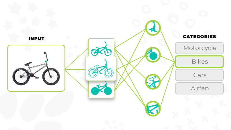
If you are trying to create a model for classifying images and have a set of examples for training, you should try a convolutional neural network. Knowing that training a convnet could be somehow struggling, I wrote this blog to help you in your first touch with this technology. Here, I will teach you how to train a customized convolutional neural network for image classification.
The repository
First of all, you will need to download our convolutional neural network repository, which is based on Tensorflow2.3 with Keras. In this repository, you will find implementations of well-known architectures like AlexNet and ResNet. Moreover, to facilitate the data manipulation, we will store it as tfrecords (a nice format of Tensorflow) that are then read by a Dataset object. This allows the model to accelerate the reading process during training.
The example dataset
To make this example easy, we will use the well-known MNIST dataset during this blog. Please download the training and testing datasets. It consists of 60000 images for training and 10000 images for testing. Figure 1 shows a sample of the images we can find in the MNIST dataset.
If you want to try with a smaller dataset, you can use MNIST-5000, which is a sample of MNIST with 5000 images for training.
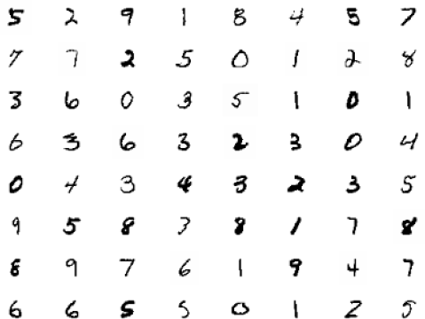
Figure 1. A sample of images from the MNIST dataset.
Prepare the dataset for training
Prepare a configuration file
- NUM_EPOCHS: The number of epochs the training will run.
- NUM_CLASSES: The number of classes in the classification task.
- BATCH_SIZE: The size of each batch.
- VALIDATION_STEPS: The number of iterations required to cover the validation dataset. It can be calculated as the size of the validation dataset divided by the batch size.
- LEARNING_RATE: The learning rate value or the initial learning rate in case of using decay schedule.
- SNAPSHOT_DIR: A path where weights are stored during training.
- DATA_DIR: The path where train.txt and test.txt are located.
- CHANNELS: The number of channels for the input images.
- IMAGE_TYPE: It is a name defining the
preprocessing operations to be applied to the input images. - IMAGE_WIDTH: The target image width.
- IMAGE_HEIGHT: The target image height.
- SHUFFLE_SIZE: It is a number representing the size of memory reserved for shuffling the data for each epoch.
- CKPFILE: It is an absolute path identifying a checkpoint from which weights are loaded for initialization. It is optional
These parameters define one experiment but we can include different sets of parameters for various experiments. To identify each set of parameters we use a section name. An example of a configuration file (mnist_full.config) that we will use for the MNIST dataset is shown below:
[MNIST]
- NUM_EPOCHS = 10
- NUM_CLASSES = 10
- BATCH_SIZE = 128
- VALIDATION_STEPS = 78
- LEARNING_RATE: The learning rate value or the initial learning rate in case of using decay schedule.
- SNAPSHOT_DIR = <PATH>
- DATA_DIR = <PATH>
- CHANNELS =.1
- IMAGE_TYPE = MNIST
- IMAGE_WIDTH = 31
- IMAGE_HEIGHT = 31
- SHUFFLE_SIZE = 10000
Create tfrecords
An efficient way to store the data is through tfrecords. This allows the data to efficiently feed the underlying neural network. In our example we create the tfrecords file using the following command:
$python datasets/create_tfrecords.py -type all -config configs/mnist_full.config -name MNIST
Train your own model
With the outputs produced by the previous step, we are ready to train the model. We define a simple architecture composed of two convolutional layers at the beginning, and two fully connected layers at the end. The last layer is the classification layers with as many neurons as classes the task has. The implementation of this architecture can be found here.
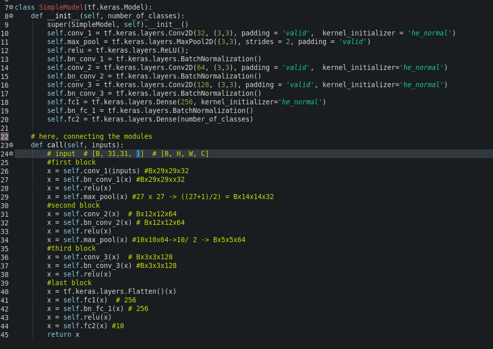
Figure 2. An implementation of a simple convnet for MNIST.
Now we are ready to train our model. You can do it running the following command:
$python train_simple.py -mode train -config configs/mnist_full.config -name MNIST
At the beginning of the execution, you will see a report of the involved parameters. Then, you will see the performance of the training for each iteration showing the loss and accuracy of the model. At the end of each epoch, the same metrics are reported for the testing (validation) dataset.
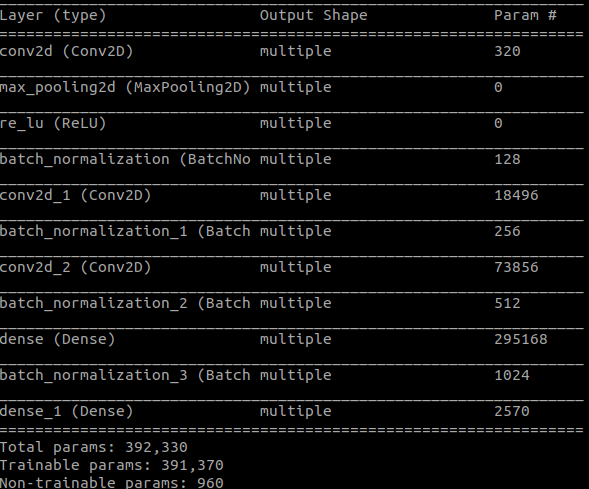
Figure 3. Parameters required for the network.

Figure 4. Output produced during training.
The training process will yield checkpoints after each epoch. In this particular case, you will see 10 files named from 001.h5 to 010.h5
Test your own model
You can also test your model. To this end, you need to set the CKPFILE parameter in the configuration file with the checkpoint you want to try (e.g. 010.h5), and then run the command below, which is very similar to the previous one changing the parameter mode for testing.
$python train_simple.py -mode test -config configs/mnist_full.config -name MNIST

Figure 5. Output produced by testing.
Predict with your trained model
$python train_simple.py -mode predict -config configs/mnist_full.config -name MNIST
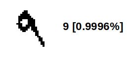
Figure 6. Example of a prediction of the MNIST model.
Understanding the code
The code in train_simple.py is composed of the following sections:
Data loading
In this section, the tfrecord file is fed into a dataset object, which allows us to organize the data into batches, apply data augmentation using the function map, and shuffle the data after each epoch.

Define callbacks for saving checkpoints
Here, we configure a ModelCheckpoint object to save checkpoints after a certain number of iterations during training (e.g., after each epoch). Check the ModelCheckpoint object for more details.

Create an instance of your network
Here, we create an instance of the network you will use. In this example, we create an instance of SimpleModel. The last part of this section builds the model defining the input size.

Loading pre-trained weights
Optionally, you can load pre-trained weight using the function load_weights of the model.

Defining the optimizer
In this section, you need to define the optimizer for your model. In this example, we are using SGD with Nesterov momentum.

Train, test or predict
