

Object detection is a common problem when it comes to computer vision. Knowledge and understanding in this area, however, is maturing rapidly, mainly because of advances in deep-learning models. The goal of object detection is to pinpoint and classify objects of interest appearing in an image. This task is naturally more complex than straightforward image classification because there may be a range of objects we are focused on, as well as the additional requirement of needing to predict bounding boxes that will encompass the detected object. A bounding box is defined by four parameters [x, y, w, h], where the first two parameters (x,y) indicate a reference spatial position in the box, commonly the center of the box or the upper-left corner, and the last two are set for the width and height of the box, respectively. An example of this task is showed in Figure 1.
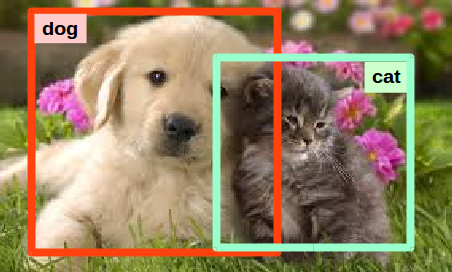
Figure 1. Object detection in action.
Deep-learning based models, through convolutional neural networks, have had a positive impact on advances in this area, and this has already led to the technology being applied to industry models. In this post, we will discuss two of the main strategies for addressing object detection. The first one is a two-stage based approach mainly represented by the Faster-RCNN [1] architecture, and the second one is a one-stage approach represented by YOLO [3].
Before the emergence of deep-learning, the task of object detection was addressed by means of a costly strategy known as “the sliding window”, where a rectangle with different sizes would move over the whole image trying to find relevant objects. For this purpose, a classifier for each of the classes we were interested in needed to be applied for each window. It was highly costly! Nowadays, state-of-the-art methods for object detection rely on a convolutional neural network which also implements a sliding window approach but in a more efficient way. Convolution layers are key!
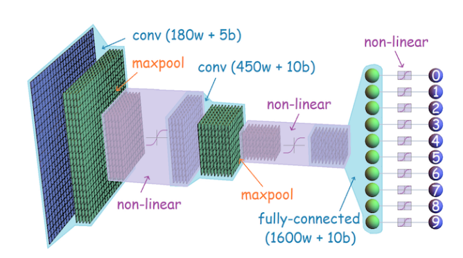
Figure 2. Scheme of a convolutional neural network [copyright Serengil].
1. Convolutional Neural Networks
A convolutional neural network (CNN) is a special kind of neural network (see Figure 2) mainly focused on processing image data but it also includes extensions to other kinds of signals which can be thought as a 2-D grid of pixels. The term convolution indicates that the network is composed of layers resembling the convolution operation used frequently in image processing. Convolutional networks are the most successful examples within the connectivist branch of the machine learning field. This can be seen as a simplified, cartoon view of brain function, sharing some properties with the primary visual cortex V1.
- V1 and CNN are arranged in a spatial map where each neuron is affected by a local receptive field. Each neuron of a convolution layer is affected by a local region in the input image, this region is known as the receptive field.
- V1 and CNN contain simple and complex cells which allow for the learning of a hierarchical representation from images. Indeed, the shallow layers in a CNN learn low-level features, similar to the well known Gabor filters, while the deeper layers bring more semantic information.
As a convolutional neural network is capable of learning highly-discriminative features, we can exploit the learned features in other problems that may be different from the classification one. In fact, we have seen successful results on similarity search, object detection, face recognition, image segmentation, image captioning, among others.
Focusing on the object detection problem, there have been significant advances in the last few years, particularly since the publication of Faster-RCNN, which brought two specific contributions: i) the use of a regions proposal network, and ii) the use of anchors to deal with the variable size of objects. A performance evolution on the object detection problem is showed in Figure 3.

Figure 3. Performance Evolution on Object Detection [copyright Girshick]
2. An end-to-end Convolutional Neural Network for Object Detection
Faster-RCNN proposed by Ren et al. [1] was one of the first proposals aiming to utilize an end-to-end trained convolutional model for the object detection problem. This proposal came up as an improvement of Fast-RCNN, a previous work which required a list of candidate objects generated by a separated module known as the objectness module. To this end, the selective search approach [5] was commonly used. Having an extra module for acquiring object candidates would mean additional costs. Therefore, the main objective of Faster-RCNN was to reduce this overhead by a convolutional architecture trained end-to-end for the object detection task.
Faster-RCNN is composed of two blocks sharing a backbone. This in turn aims to produce discriminative features that will be used to estimate candidate objects as well as to predict the class of those objects. Of course, the backbone is also a convolutional neural network! To this end, a ResNet architecture has recently been used. The first block, termed Region Proposal Network (RPN), is devoted to find regions where an object is highly likely to appear, while the second block is just the Fast-RCNN focusing on predicting the class of proposed objects.
2.1. Region Proposal Network
The Region Proposal Network (RPN) is a convolutional network devoted to detect regions in the image where objects may be found. This works as a class-agnostic stage.
The backbone of the RPN is a convolutional neural network. To this end, a ResNet arquitecture has been recently used. The deeper convolutional layer is used as the feature map and this map is arranged into HxW nodes. Each node is related to a receptive field with a certain size in the input image. The exact size will depend on the feature map depth.
The RPN places a convolutional layer immediately after the feature map, aiming to learn 256 features for each node. This is carried out by simply connecting a 256-channel convolutional using a 3×3 kernel. The result of this layer is the new feature map that will be used to predict the occurrence of an object.
The last component of the RPN is the predictor. Actually, we have two kinds of predictors, one in charge of predicting whether a region contains an object or not, and the other in charge of predicting the bounding box covering the object, if it occurred. The first one is a kind of classifier, while the second is a regressor.
To accelerate the training, RPN uses a set of reference regions per node, the anchors, which actually represents a rectangular region in the input image which is positioned in the center of the receptive field with respect to each node in the feature map. An anchor is defined by its scale (e.g. 64×64) and its aspect ratio (e.g. 1:1, 1:2, 2:1). The choice of the anchors (scale and aspect ratios) strongly depends on the application being used. In the Figure 4, a set of anchors is illustrated.

Figure 4. Examples of anchor for a node.
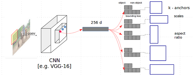
Figure 5. RPN Arquitecture
Supposing we have defined K anchors per node, the classification block will need to learn 2K classifiers. That is, it will learn an object-classifier as well as a non-object classifier per anchor. On the other hand, the regressor will learn four parameters per anchor. These parameters represent certain transformations that an anchor must undergo to tightly cover the objects with respect to the four parameters which define it. Therefore, the number of regressors that RPN needs to learn is 4K. In Figures 5 and 6, the RPN architecture is shown. For training, the classifier set uses a classical cross-entropy loss, while the regressor set uses the smooth-L1 loss function.
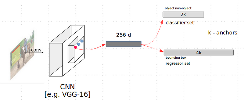
Figure 6. 2K classifiers and 4K regressors in the RPN
2.2. Detection by Fast-RCNN
This is the second block of the Faster-RCNN, and actually this corresponds to the Fast-RCNN model. However, in this case, the set of candidate objects will be provided by the RPN block. The Fast-RCNN is focused on predicting the most probable class (given a set of predefined classes) plus an extra class representing the background. For this purpose, the model again depends on a convolutional neural network to provide discriminative features for each region of interest (ROI). This is the backbone of the model and it is the same as that used by the RPN block.
Having a feature map computed from the input image through the convolutional backbone, the Fast-RCNN extracts a subregion according to the candidate ROIs proposed by the RPN. We must be aware that the diversity of sizes within the area of interest is really a matter of defining the architecture of a convolutional model. To address this problem, Fast-RCNN proposes a special layer termed “ROI Pooling Layer” which, through an average pooling operation, transforms the feature map with respect to a given ROI into a feature map of HxW nodes. The result is then passed through a couple of fully connected layers to finally pass to a set of classifiers to predict the most probable class, as well as to a set of regressors in charge of adjusting the input ROI using semantic information. In Figure 7, a scheme of Fast-RCNN is shown.
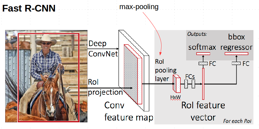
Figure 7. Fast-RCNN (image from original paper[2])
3. Toward Real Time Detection with YOLO
The two-stage based approach proposed by Faster-RCNN is the main drawback of the model. It would be more efficient if a one-stage approach could do the same work, right? Well, YOLO [3] has been proposed to address this drawback. In fact, YOLO is an acronym of the expression “You Only Look Once”.
The first proposal via YOLO is somewhat minimalist, which also makes it attractive. Like Faster-RCNN, the backbone of the proposal is a convolutional network which produces a feature map from an input image. This feature map contains SxS nodes, each one related with a receptive field in the input image. Each node also predicts B bounding boxes as well as a score for each box. This score represents how confident a model is about finding an object in that box. A score of zero will mean that there is no object in the box. Consequently, five predictors are required for each bounding box. These predictors estimate the (x,y) coordinates representing the center of the box, the width (w) and height (h) of the box as well as the confidence of the prediction. In addition, each node also predicts C conditional class probabilities P(C_i | Object). The proposal predicts one set of class probabilities per each node, regardless of the number of boxes. Therefore, at the end, the model needs to estimate (SxSx(Bx5 + C)) regressors as showed in Figure 8.
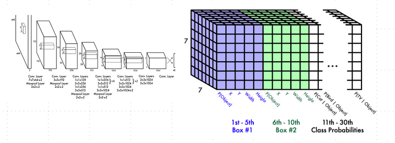
Figure 8. YOLO in action. The colored volume represents the set of learned regressors.
Although, the prediction speed of the model is very high, the performance is not yet comparable with Faster-RCNN, undergoing a poor localization. However, in the follow-up version of YOLO[3] (YOLO9000 [4]), the authors incorporated the use of anchors which then allowed them to improve the localization.
In the last year, there have been other improvements focused on powering up the performance of one-stage models leveraging the multi-scale information embedded into the convolutional neural nets and addressing the class imbalance present within the object detection problem. However, these new improvements will be discussed in the next posts.
References
[1] Shaoqing Ren, Kaiming He, Ross Girshick, Jian Su. nFaster R-CNN: Towards Real-Time Object Detection with Region Proposal Networks. https://arxiv.org/abs/1506.01497
[2] Ross Girshick, Fast R-CNN. https://arxiv.org/abs/1504.08083
[3] Joseph Redmon, Santosh Divvala, Ross Girshick, and Ali Farhadi. You Only Look Once: Unified, Real-Time Object Detection. https://pjreddie.com/media/files/papers/yolo_1.pdf
[4] Joseph Redmon, Ali Farhadi. YOLO9000: Better, Faster, Stronger. https://pjreddie.com/media/files/papers/YOLO9000.pdf
[5] J. R. R. Uijlings, K. E. A. van de Sande. T. Gevers. A.W.M.Smeulders. Selective Search for Object Recognition
